T test in Excel for Hospital Performance Data: Running the T Test
Post 2:
In the first blog post of this series, I introduced the idea of using Excel to run T test on hospital quality data from CMS Hospital Compare. I laid out the assumptions and approach to the analysis. Please check it out before proceeding.
The focus of this blog is setting up the Excel sheet with data and entering in the formulas to run the analysis. As noted in the prior blog, the CMS Hospital Compare measure that we’ll use for this analysis is: “Median Time from ED Arrival to ED Departure for Admitted ED Patients”.
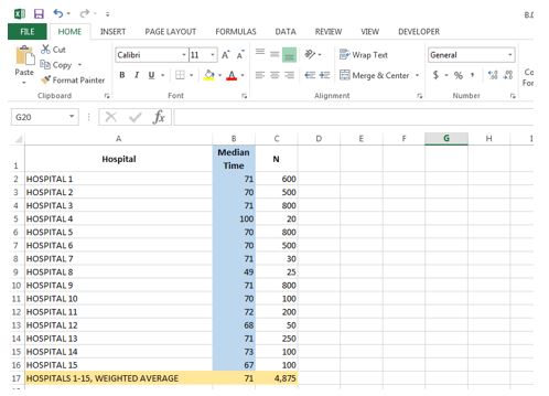
- Bring in the following data into Excel- Hospitals in your comparison, the performance results (median time in minutes), and the weighted average. It is optional to add in the sample sizes for each hospital (N), but it is only needed to calculate the weighted average.

Column A lists the Hospitals in the comparison, Column B shows the median time from ED arrival to ED departure for each hospital, and the Column C provides the sample size for each hospital, which in this case is the number of ED admits (the admit numbers are unreasonably high, but as noted, this data is made up for the sake of the example).
The weighted average for the 15 hospitals is in Row 17. To calculate the weighted average in Cell B17, you’d take the sum of all the products between the cells in Column B and the cells in Column C (B2*C2 + B3*C3 + … + B16*C16) and divide by the sum of the cells Column C (C2 + C3 + … + C16). In Excel, this would be achieved by the following formula in Cell B17:
=(SUMPRODUCT(B2:B16, C2:C16))/SUM(C2:C16) (1.1)
- Calculate number of hospitals, standard deviation, and degrees of freedom

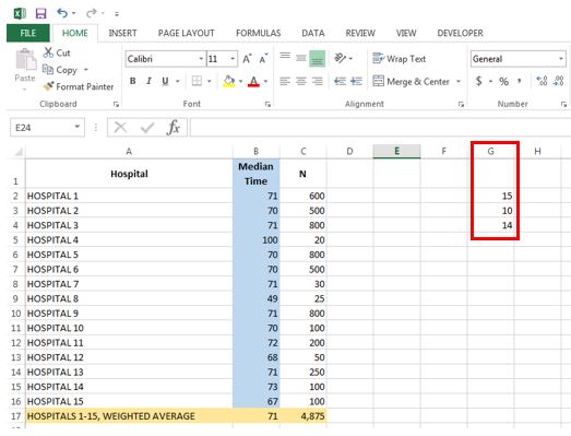
I do this in Column G.
Cell G2 tells us the number of hospitals; while we can easily count up 15 hospitals, I prefer to derive it formulaically to reduce human errors, using the following line:
=COUNTIF(B2:B16, “<> “) (2.1)
The formula above ensures I’m not counting any blank spaces. Perhaps this is overkill, but it again is an easy way to mitigate occurrence of errors. I find the standard deviation in Cell G3:
=STDEV(B2:B16) (2.2)
I then calculate the degrees of freedom in Cell G4, which is simply equal to the number of hospitals minus one:
=G2-1 (2.3)
- Perform T test, obtain p-value, and determine statistical significance

I run the T test in Column D. The formula I use for Cell D2 is:
=TDIST(ABS((B2-B$17)/G$3), G$4, 2) (3.1)
The formula first finds the z-score of Hospital 1’s performance in Cell B2 from the following: (B2-B$17)/G$3. I use the ABS() function to find the absolute value, as Excel will not apply T test to a negative value. I then apply the T test with the TDIST() function with the degrees of freedom from Cell G4 and with tails set to “2”. Doing so gives me the p-value for Hospital 1. Lastly, I apply this formula to all other rows by clicking “Copy” on Cell D2 and then “Paste” onto Cells D3 to D16.
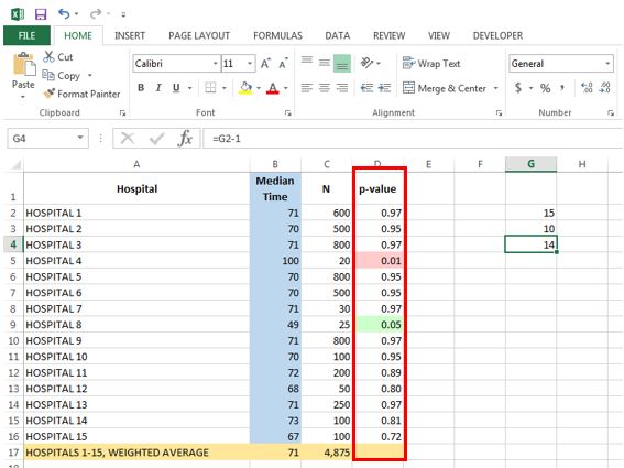
Column D is now populated with the p-values for each hospital based on the T test. By finding the cells where p-values are less than or equal to 0.05, we can now determine which hospitals performed statistically different from the average.
To add an aesthetic kick, I utilize Excel’s conditional formatting option to highlight cells in Column D as green where p-values indicate that a hospital is a significantly better performer than the average and as pink where the p-values indicate a significantly worse performer. In this case, a lower median time indicates better performance, and we find that Hospital 8 is a significantly better performer than the average, whereas Hospital 4 is significantly worse performer with a higher median time than the average.
